External Resources

Kilian Weinberger’s SVM Lecture Notes An excellent, concise, comprehensive look at SVMs. Less gradual than the two resources below, but on the flipside very to-the-point.
Support Vector Machines (SVM) — An Overview provides a good overview of SVMs/parameters, as well as a straightforward example of a kernel transformation
Support Vector Machines explained with Python examples provides a more in-depth exploration of SVMS and some of the math, as well as providing some good Python examples

Support Vector Machines

Introduction

The basic premise behind Support Vector Machines (SVMs) is that they provide a supervised method for finding an efficient binary classifier. Specifically, given a set of labelled vectors in n dimensions, we find a line/plane (linear equation) in n-1 dimensions that best partitions our vectors.

We will start by talking about maximum/hard-margin SVMs, used for data that is linearly separable, i.e. that can be split by a line. A more comprehensive introduction to linear separability can be found under Linear Classifiers, if desired. We will then talk about an extension of them that can be used for non-linearly-separable data.

Maximum-margin SVMs

Motivating Example

To give an example, we might have red (square) vectors and blue (circle) vectors, and desire a simple way of determining what’s what. The green line/hyperplane in the below image splits them in twain, and we can thus derive an expression that takes in a vector and results in different labels - negative values on one side of the line and positive values on the other.

separating boundary image

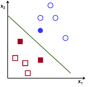
For example, one might imagine the equation of the line here is some $\vec{w}\cdot\vec{x} - b = 0$ - in that case, we can let our classifier function be $\texttt{sgn}(\vec{w}\cdot\vec{x} - b)$ , resulting in -1 for vectors below the line and +1 for vectors above the line.

Choice-of-Hyperplane Intuition

In the previous example, the demonstrated line actually is the result of running a support vector machine. But why that line? Consider the example again, at left, and the figure at right.

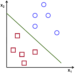
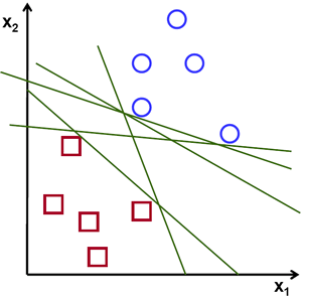
separating boundary image nonoptimal separating boundaries image

All of these green lines separate the vectors properly, and indeed could all be used to generate equations for determining the vectors’s labels. The line on the left, though, maximizes the distance to the closest sample in each class, and so typically generalizes best to out-of-sample data.

Sure, we could have some wonky underlying distribution, such as where the circles actually appear really close to the squares (or even within the cavity of the squares), but with the information we know (i.e. our collection of samples) additional justification would be needed for choosing anything but this line.

Looking at the line again, we’ve highlighted the closest vectors, known as the support vectors as well as indicated what we mean when we say “maximizing the distance to the closest sample in each class”, also known as the margin.

maximizing margin image

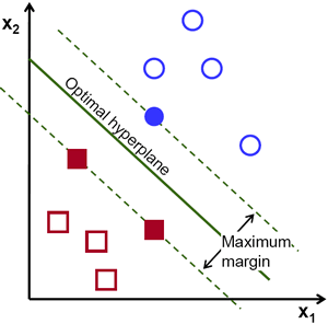
The margin can be imagined as a sort of street, where the separating hyperplane is the median and the the lines passing through the support vectors are the curbs.

Support Vector Intuition

Notice that, as the optimal hyperplane is that which separates the classes and maximizes the margin to the closest vectors (aka the support vectors), the optimal hyperplane is entirely defined by the support vectors. The support vectors are alternatively given as the collection of vectors that lie on the margin boundary (take a moment to convince yourself that these are the same).

Maximum-margin Hyperplane Equation

The maximum-margin hyperplane equations out there can seem a little opaque, so we’ll build it up intuitively. Recall that our goal is to select a line/plane that maximizes the margin about it, that is, a line/plane that is the furthest from any of the datapoints subject to separating them. The format for the equation for this, then, is

$\textup{Line/plane with greatest distance to datapoints} \textit{ that} \textup{ separates the classes}$

For the purposes of the equation, we formalize our set of inputs-output pairs as $\{(\vec{x}_i, y_i)\}$ , where $\vec{x_i}\in \R^d$ and (giving the output labels values of -1 and 1 for the sake of computation) $y\in\{-1, 1\}$ .

Finding the maximum-margin hyperplane described by some line/plane $P = \{\vec{x}\in \R^d \textit{ such that } \vec{w}^T \vec{x} + b=0\}$ then becomes

$(\vec{w}^*, b^*)= \underbrace{ \arg\max_{\vec{w}, b}\hspace{6} \underbrace{ \min_{i} \frac{\left|\vec{w}^T\vec{x}_i + b\right|} {\|\vec{w}\|} }_ { \textup{distance to closest } \vec{x_i} \textup{ vector} } }_ { \textup{Margin that maximimizes distances to vectors} } \textit{such that } \underbrace{ \forall i, \ y_i(\vec{w}^T\vec{x}_i+b) \geq 0 }_ {\textup{The hyperplane is separating} }$

The problem of finding which then boils down through some very nontrivial simplifications to

$(\vec{w}^*, b^*)= \underbrace{ \arg\min_{\vec{w}} \|\vec{w}\| }_ { \textup{Margin that maximimizes distances to vectors} } \textit{such that } \underbrace{ \forall i, \ y_i(\vec{w}^T\vec{x}_i+b) \geq 0 }_ {\textup{The hyperplane is separating} }$

Notice that the goal is to minimize $\|\vec{w}\|$. This can also be a thought of another way - in fact, because of how hard-margin SVMs are trained, the expression for the margin is $\frac{2}{\|\vec{w}\|}$ (and the distance from the separating hyperplane to one of those points is relatedly $\frac{1}{\|\vec{w}\|}$). As such, since the goal is to maximize the margin ($\frac{2}{\|\vec{w}\|}$), that same goal is to minimize $\|\vec{w}\|$.

Soft-Margin SVMs (for non-linearly-separable data)

Not all data is linearly separable, however. For data that isn’t linearly-separable, maximizing the margin does not necessarily minimize the error. To accommodate for this, soft-margin SVMs use what’s called a slack parameter, C, that can be tweaked to prioritize how much we want to maximize the margin versus how much we want to minimize the error.

Now, you might be asking at this point what the meaning of a margin even is if there’s no separating hyperplane. To address this, we use the equation we derived earlier as a description of “maximum margin”-ness and penalize the result using the error by a factor of C.

Soft-Margin Hyperplane Equation

$\begin{align*} ( \vec{w}^*, b^*, \vec{\xi}^*) = \arg\min_{ \vec{w}\in\R^d, b\in\R, \vec{\xi}\in\R^N} \ & \frac{1}{2} \| \vec{w}\|^2 + C\sum_{i=1}^N \xi_i \\ \mbox{s.t. }\ & y_i(\inner{ \vec{w}^T}{ x_i} + b) + \xi_i \geq 1, \quad i=1,\dots,N .\\ & \textup{(all } \xi_i\textup{ being nonnegative)} \end{align*}$

Okay, so I lied a little bit by virtue of neglecting to mention ξ. Each ξᵢ just represents to what degree it is that you’re willing to be incorrect for your prediction for a given input vector xᵢ. However, by letting C ≥ 0, you can ignore ξ entirely (minor COVID-19 perk- I don’t need to write this for you all on a whiteboard*) and convert this into

$\begin{align*}(\vec{w}^*, b^*) \hspace{5}=\hspace{5} \arg\min_{\vec{w}\in\R^d, b\in\R}\underbrace{ \frac{1}{2} \|\vec{w}\|^2 }_{\textup{Maximizing margin}} \ + \hspace{5} C\underbrace{\sum_{i=1}^N \begin{array}{cc} \ 1-y_{i}(\vec{w}^T \vec{x}_{i}+b) & \textrm{ if $y_{i}(\vec{w}^T \vec{x}_{i}+b)<1$}\\ 0 & \textrm{ if $y_{i}(\vec{w}^T \vec{x}_{i}+b)\geq 1$} \end{array}}_{\textup{Penalization/loss due to errors}} \end{align*}$

Which then can be written as

$\begin{align*}(\vec{w}^*, b^*) \hspace{5}=\hspace{8} \arg\min_{\vec{w}\in\R^d, b\in\R} \hspace{10} \underbrace{ \frac{1}{2} \| \vec{w}\|^2 }_{\textup{Maximizing margin}} +\hspace{15} \ C\underbrace{\sum_{i=1}^N \max(1-y_{i}(\vec{w}^T \vec{x}_{i}+b),\ 0) }_{\textup{``Hinge loss'', penalization due to errors}} \end{align*}$

* A meme about how hard the Greek letter Xi is to write