External Resources

Predrag Radijovac and Marth White’s Machine Learning Handbook
Much of this page was directly patterned after sections 1.1-1.4 of this book, which was used to teach this course in a previous semester.

Probability

Samples and Events

Probability deals with outcomes, the results that can and do happen in our world. We’ll give some formal definitions to begin with, then flesh them out with a real-world example.

Definitions

Formally, we refer to tiny discrete outcomes as samples. We refer to collections of those samples as events. Samples are drawn from the set of all samples, the sample space Ω; events are drawn from the set of all events, the event space ℰ, and (for finite sample spaces) events are just collections of outcomes, ℰ = set of all possible sets of samples, 𝒫(Ω), the power set of Ω.

Example

As an example, suppose you’re rolling a six-sided dice. The samples space here is Ω={1, 2, 3, 4, 5, 6}. The event space, meanwhile, is all the ways you could get some number of these samples - ℰ={ {}, {1}, {2}, {3}, ..., {1, 2}, {1, 3}, ..., {1, 2, 3, 4, 5, 6} }. By focusing on the event space, this not only lets us talk about “hey, look, I rolled a 3” - the event {3} - but also more complicated situations, like “hey, look, I rolled an even number” - the event {2, 4, 6}.

Axioms

The event space ℰ must satisfy that

If an event A is in ℰ, then Aᶜ is in ℰ. In other words, $A \in \mathcal E \Rightarrow A^c \in \mathcal E$
If a collection of events A₁, A₂… is in ℰ, then the set of all their constituent samples ∪(A₁, A₂…) is an event in ℰ. In other words, $A_1, A_2, ... \in \mathcal E \Rightarrow \left(\bigcup A_1, A_2 ...\right) \in \mathcal E"$
There is at least one event. In other words, $|\mathcal E|>0$

A space (Ω, ℰ) is known as a measurable space.

Example 2: Electric (Burnout) Boogaloo

Suppose we are owners of a “Braum’s Ice Cream” shop (a popular chain in Oklahoma, USA), and we have a large neon sign in front of our store.

Neon "Braum's Ice Cream" sign. The letters B R A U M and S are lit up

If we consider the outcomes of our lights going out, we have a sample space Ω={B R A U M S}, with each letter corresponding to the light going out. Our events would then be which collection of lights go out - naturally, for example, if we have the event A={R A U M S}, we just have ‘B Ice Cream and Dairy Store’. There are certain events we naturally want to avoid - for example, the event A={B A M S} = {R U M}ᶜ - the event where the letters B, A, M, and S go out, or the complement of the event where R, U, and M go out - would just leave us with ‘RUM Ice Cream and Dairy Store’. A similar unfortunate event is given below.

Neon "Braum's Ice Cream" sign. The letters B R and A are lit up

Exercise: briefly think through what the sample space/event space would be for the lights of a a Snap Fitness™ location (and what events you might want to avoid if you were responsible for it).

Neon "Snap Fitness" sign. The letters N A and P are lit up, followed by "Fitness"

Probability Distributions

Another example of having an event space is that it allows us to derive probabity distributions. A probability distribution is, formally, a function P:ℰ⟶[0, 1] from events to the range 0-1 inclusive if

$P(\Omega)=1$ (the probability of any of the samples occurring is 1)
$\forall A_1, A_2\in \mathcal E, (A_1\cap A_2 = \emptyset) \Rightarrow P(A_1 \cup A_2) = P(A_1) + P(A_2)$ (for two disjoint events, the probability that any of their aggregate samples occur (the probability either event occurs) is the same as the sum of the probabilities of the two events)

Discrete Example

Consider modelling the probabilities of the roll of a die. The sample space is the finite set Ω = {1, 2, 3, 4, 5, 6} and the event space ℰ is the power set P(Ω) = {∅, {1}, {2}, . . . , {2, 3, 4, 5, 6}, Ω}, which consists of all possible subsets of Ω. A natural probability distribution on (Ω, E) gives each die roll a 1/6 chance of occurring, defined as P({x}) = 1/6 for x ∈ Ω, P({1, 2}) = 1/3 and so on.¹

The first property just tells us that the event “the die roll is 1, 2, 3, 4, 5, or 6” is 100% likely to happen. For the second property, consider the event “the die roll is 2 or less” - A₁={1, 2} - and the event “the die roll is 5 or more” - A₂={5, 6}. The second property tells us that, since A₁ ∩ A₂ = {}, P(A₁) + P(A₂) = P(A₁ ∪ A₂). In other words, the second property tells us that P(“getting a die roll ≤ 2 or a die roll ≥ 5”) = P(“getting a die roll ≤ 2”) + P(“getting a die roll ≥ 5”).

These properties can be readily used to derive other facts about probability distributions as well - such as that P(Aᶜ) = 1-P(A).

Continuous Example

Consider modelling the probabilities of the angle of a dart thrown against a dartboard. The sample space is the continuous interval Ω = [0, 360] (which is an infinite set). The event space for continuous sets is more complicated than what we’ve discussed (it’s not simply the power set of Ω - it’s a subset of that), but for this example, it’s the collections of continuous intervals you can form of angles on a dartboard - so, for example, A=[0, 90]∈ℰ would be a quarter of the dartboard, as would A=[330, 60]∈ℰ.

Dartboard with some angles highlighted. Specifically, dartboards are split up into radial pieces, and the highest-scoring radial piece extends from the center to the top of the board, bordered by lines along the angles 261 degrees and 279 degrees (the 18 degree sector centered on the line extending from the center to the top of the board)

You might imagine that a really good player (who didn’t aim for the center) would have a probability distribution that had higher values for intervals between 261 degrees and 279 degrees. Unlike in the discrete case, deriving a probability distribution P here is tricky, as we Naturally, describing this probability distribution might be a bit tricky- we have have to define outputs for the intervals in the sample space! - thankfully, as we shall see, we don’t need to focus overmuch on the formal definition of a probability distribution to effectively define one.

Probability Mass & Density Functions

Probability distributions themselves are a bit daunting to consider directly - it can be useful to be able to fall back on their technical sense, but that same sense is unwieldy to work with. Fortunately, we can instead obtain probability distributions by simply defining them in terms of probability density functions and probability mass functions.

Probability mass/density functions rely on defining a density value at each point in the sample space - probabilities of items in the event space are then the sum/integral of their constituent samples. It’s worth noting that PMFs and PDFs don’t necessarily produce probabilities (although for spaces of finite size (cardinality) they do).

Probability Mass Functions

For a discrete sample space Ω, a PMF is a function $p:\Omega \to [0, 1]$ that satisfies

$\displaystyle\sum_{\omega\in \Omega}{p(\omega)}=1$

PMF Example

Consider our six-sided die from earlier, where the sample space is Ω = {1, 2, 3, 4, 5, 6}. We could have many underlying distributions, but assuming a fair die (a.k.a. unweighted) we have

$p(\omega) = \frac{1}{6}$

Using, this, if we wanted to find the probability of rolling an odd number, we could do P({1, 6}) = p(1) + p(6) = 1/6 + 1/6 = 2/3. The distribution defined by this PDF is known as the discrete uniform distribution.

This generalizes to more complicated situations- in the event there was some more complicated underlying distribution, like if someone was cheating with a weighted die, we could also use a PMF to model that.

Probability Density Functions

For a continuous sample space Ω, a PMF is a function $p:\Omega \to [0, 1]$ that satisfies

$\displaystyle\int_{\omega\in \Omega}{p(\omega)}=1$

PDF Example

Suppose you have a random number generator that outputs numbers between 10 and 50, inclusive, with equal probability. The distribution here is known as the continuous uniform distribution, and the equation governing its PDF is given by

$p(\omega)=\frac{1}{40}$

Exercise: Considering what you know about how a PDF works, see if you can derive the continuous and discrete distributions for arbitrary starting and ending values for the sample space.

Using PDFs and PMFs

PDFs and PMFs can be used for a variety of purposes, including finding the probability of an event occurring and finding the mean value for a distribution.

Using our previous uniform RNG example, $P(15 \leq X \leq 20)$ , for example, is

$\displaystyle\int_{15}^{20}p(x)\ dx = \left[\frac{x}{40}\right]_{15}^{20} = \frac{5}{40}$

And the average (mean) value for the the whole distribution is

$\displaystyle\int_{10}^{50}x\cdot p(x)\ dx = \left[\frac{x^2}{80}\right]_{10}^{50} = 30$

Random Variables

Frequently, you will see P(X=x) or the like. The X is in this case is what’s known as a random variable. Random variables are ‘variables’ that take on values in the sample space with some underlying distribution. $P(X=\textup{whatever})$ just asks what the probability is that X will take on the value/satisfies whatever.

For example, in the case of a fair die I might have a random variable that samples from Ω={ 1, 2, 3, 4, 5, 6 } with equal probability. In that case, X is a random variable sampling from a uniform distribution over the sample space, and $P(X=1)=\frac{1}{6}$ .

As a formal note, random variables are technically transformative functions, which is why, for example, $P(X=\textup{even})=\frac{1}{2}$ is also valid. However, in practice we do not think of underlying functions when working with random variables, and just think of them as variables that satisfy properties/match values.

Expected Values

The expected value $\mathbb{E}[X]$ of a random variable X is the mean/average of repeatedly sampling X. In the case of X representing our fair die roll, $\mathbb{E}[X]=3.5$ .

More generally, the expected value of a random variable is given by the following equations:

$\mathbb{E}[X]= \begin{cases} \displaystyle \sum_{x \in \Omega} x p(x),& \text{if } X \text{ is sampled from a discrete space}\\ \displaystyle \int_{x \in \Omega} x p(x), & \text{if } X \text{ is sampled from a continuous space} \end{cases}$

In other words, the expected value is the result of adding up each of the samples by their weight of occurrence. In the below spinner, if we have a random variable representing the underlying distribution of spin results, the expected value is just each result weighted by its odds of occurring.

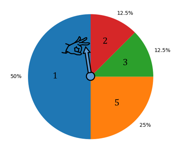$E[X] = 0.5 * 1 + 0.125 * 2 + 0.125 * 3 + 0.25 * 5 = 2.375$

Independence and the Product Rule

First and foremost, if X and Y are random variables, their joint probability is the probability that both result in specific events. The joint probability that X results in outcome x and Y results in outcome y is written as P(X=x, Y=y) or p(x, y) .

Two random variables X and Y are independent if their outcomes do not depend on each other in any way. If X and Y are independent variables, then their joint probability is just the product of the individual probabilities, i.e.

p(x, y)=p(x)p(y)

which is known as the product rule for independent random variables.

Conditional Probability

For two random variables X and Y sampling from event spaces $\mathcal X$ and $\mathcal Y$ , the conditional probability of an event $x\in \mathcal X$ occurring on an event $y \in \mathcal Y$ occurring is written as either P(X=x | Y=y) or p(x|y)

The basic idea is to ask “if we know that y occurred, what is the probability that x will occur?”. The equation for this is

$p(x|y) = \frac{p(x, y)}{p(y)}$

Put another way, the conditional probability of x on y looks at “what proportion of the time when y occurs do both x and y occur?

Two random variables X and Y are independent if and only if the conditional probability of one on the other is the same as their isolated probabilities - that is, p(x|y) = p(x) (alternatively written as P(X=x|Y=y)=P(X=x) )

More generally, for two random variables X and Y, their joint probability is given as

p(x, y)=p(x|y)p(y) = p(y|x)p(x)

which is the product rule for random variables. The product rule for independent random variables is therefore a special case of this.

Bayes’s Rule

Using the product rule for random variables, we can obtain what’s known as Bayes’s rule. Rearranging p(x|y)p(y) = p(y|x)p(x) , we get

$p(x|y) = \frac{p(y|x)p(x)}{p(y)}$

¹ Text taken nearly directly from Predrag Radijovac and Marth White’s Machine Learning Handbook at https://marthawhite.github.io/mlcourse/notes.pdf